Tables, charts and graphs are useful for representing data visually to make them more easily understandable.

Tables

Example table 1: Score of individuals at an archery game

Score	Frequency	Percentage (%)
1	0	0
2	3	60
3	2	40

Example table 2: Education level of individuals vs their annual salary

		Education
		University	Apprenticeship	High school
Salary ($)	10-49k	1	6	5
	50-99k	2	6	3
	100k+	3	2	0

Tables are useful for summarising sets of data. Common tables in epidemiology include the frequency table that present categorical, nominal or ordinal data (e.g. Example table 1). These record of how often each value (or set of values) of the variable in question occurs. It may be enhanced by the addition of percentages that fall into each category. Contingency tables are frequency tables that present more than one categorical variable, it may be called a contingency table (e.g. Example table 2).

Charts & graphs

Pie chart

A pie chart summarises categorical data. It is a circle which is divided into segments which each represent a particular category. The area of each segment is proportional to the number of cases in that category.

Bar chart

Bar charts visualise distribution across nominal or ordinal data. It displays the data using a number of bars (rectangles of the same width usually drawn with a gap between the them), each of which represents a particular category. The length of each rectangle is based on the number of cases in the category it represents. They can be displayed horizontally or vertically .

Dot plot

A dot plot illustrate the distribution of data and can help detect any outliers or any gaps in the data set. Each dot represents a fixed number of cases. For nominal or ordinal data a dot plot is similar to a bar chart, while for continuous data the dot plot is similar to a histogram, with the bars/rectangles replaced by dots in both cases.

Histogram

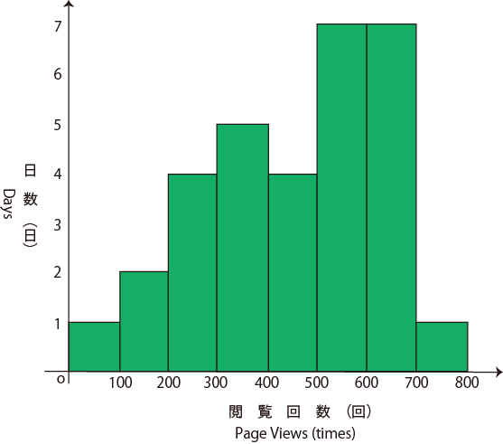
The histogram is only appropriate for discrete or continuous values measured on an interval scale (as such unlike bar graphs there is no gap between rectangles/bars). It illustrates the distribution of data and helps outliers or gaps in the data set. The range of possible values in a data set is divided into groups. For each group, a rectangle is constructed with a width corresponding to the range of values in that specific group, and a height (and thus area) proportional to the number of observations falling into that group. It is generally used for large data sets (>100 observations), when stem and leaf plots become tedious to construct.

Stem and leaf plot

A stem and leaf plot is similar to a histogram by summarising data measured on an interval scale, but usually for smaller data sets (<100 data points). It provides a table with data ordered by magnitude as well as a picture of its distribution. By using a back-to-back stem and leaf plot, we can compare the same characteristic in two different groups (e.g. height of boys and girls).

Box and whisker plot

A box and whisker plot (or box plot) is used on data on an interval scale. The picture produced consists of the most extreme values in the data set (maximum and minimum values), the lower and upper quartiles, and the median. It is especially helpful for indicating whether a distribution is skewed and whether there are any outliers. Box and whisker plots are also useful when large numbers of observations are involved and when two or more data sets are being compared.

Scatter plot

Scatter plots are used to visualise bivariate data. Each unit contributes one point to the plot. The resulting pattern indicates the type and strength of relationship between two variables. Often, variables are in a linear relationship, such that a regression line can be fitted to the graph aid to aid interpretation of the correlation coefficient or regression model. However, the variables can also be in non-linear relationships or clustered.